 This notebook is part of a GitHub repository: https://github.com/pessini/SFI-Grants-and-Awards
MIT Licensed
Author: Leandro Pessini
SFI - Gender differences in research grant applications
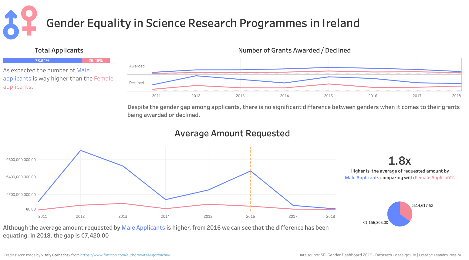
¶Gender Equality in STEM Research Programmes in Ireland

![]() This report will provide an overview of gender equality in awards applied by Science Foundation Ireland (SFI) which is the national foundation for investment in scientific and engineering research. The data provided covers a period of time between 2011 and 2018.
This report will provide an overview of gender equality in awards applied by Science Foundation Ireland (SFI) which is the national foundation for investment in scientific and engineering research. The data provided covers a period of time between 2011 and 2018.
The Agreed Programme for Government, published June 2002, provided for establishing SFI as a separate legal entity. In July 2003, SFI was established on a statutory basis under the Industrial Development (Science Foundation Ireland) Act, 2003.
SFI provides awards to support scientists and engineers working in the fields of science and engineering that underpin biotechnology, information and communications technology and sustainable energy and energy-efficient technologies.
The analysis is on gender differences in research grants offered by SFI whether the award was accepted or declined by the applicant.
Audience
A core principle of data analysis is understanding your audience before designing your visualization. It is important to match your visualization to your viewer’s information needs.
This ad hoc analysis aims to deliver a presentation to the SFI Executive staff, Director of Science for Society. The director has the responsibility for overseeing all Science Foundation Ireland research funding programs and management of funded awards.
Dataset
The dataset used is SFI Gender Dashboard 2019 and includes SFI research programmes from 2011 that were managed end-to-end in SFI’s Grants and Awards Management System and reflects a binary categorisation of gender, e.g. male or female between 2011 and 2018. For more information, check out the Data Dictionary available.
Dataset provided by Ireland's Open Data Portal which helds public data from Irish Public Sectors such as Agriculture, Economy, Housing, Transportation etc.
Libraries
# Change the default plots size
options(repr.plot.width=15, repr.plot.height=10)
options(warn=-1)
# Suppress summarise info
options(dplyr.summarise.inform = FALSE)
options(dplyr = FALSE)
# Check if the packages that we need are installed
want = c("dplyr", "ggplot2", "ggthemes", "gghighlight",
         "grid", "foreign", "scales", "ggpubr", "forcats",
         "stringr", "lubridate", "Hmisc", "psych")
have = want %in% rownames(installed.packages())
# Install the packages that we miss
if ( any(!have) ) { install.packages( want[!have] ) }
# Load the packages
junk <- lapply(want, library, character.only = T)
# Remove the objects we created
rm(have, want, junk)
sfi.grants.gender <- read.csv('../data/SFIGenderDashboard_TableauPublic_2019.csv')
head(sfi.grants.gender)
sfi.grants.gender2 <- sfi.grants.gender
sfi.grants.gender2$Award.Status <- as.factor(sfi.grants.gender2$Award.Status)
sfi.grants.gender2$Applicant.Gender <- as.factor(sfi.grants.gender2$Applicant.Gender)
sapply(sfi.grants.gender2, function(x) sum(is.na(x)))
# There are 59 NA records for Amount Requested
sfi.grants.gender2 %>% filter(is.na(Amount.Requested)) %>% group_by(Applicant.Gender) %>% summarise(n = n())
# Cleaning NA values for Amount Requested because the analysis will use this variable
sfi.grants.gender2 <- sfi.grants.gender2 %>% filter(!is.na(Amount.Requested))
sapply(sfi.grants.gender2, function(x) sum(is.na(x)))
Hmisc::describe(sfi.grants.gender2)
# By Gender
describeBy(sfi.grants.gender[,c("Amount.Requested", "Amount.funded")], sfi.grants.gender$Applicant.Gender)
As expected the number of Male Applicants is way higher than Female ones.
- Male Applicants = 2.000
- Female Applicants = 719
# Creating a category based on quantile to categorize the Amount Requested
sfi.grants.gender2 <- sfi.grants.gender2 %>%
  mutate(Category.Amount= cut(Amount.Requested,
                             breaks=quantile(Amount.Requested, c(0,.25,.50,.75,1), na.rm = TRUE),
                             labels=c("low","medium","high","very-high")))

# handling amount requested = 0
sfi.grants.gender2$Category.Amount[sfi.grants.gender2$Amount.Requested == 0] <- "low"

sfi.grants.gender2 %>% group_by(Category.Amount) %>% summarise(total= n()) %>% ungroup()
paste0("Number of rows in the dataset: ", nrow(sfi.grants.gender2))
# Filtering the total amount requested and number of request for all applicants
total_requested <- sfi.grants.gender2 %>%
summarise(Total.Amount.Requested = sum(Amount.Requested),
         Total.Requests = n())
total_requested
# Filtering the total amount requested and number of request by Gender
requests_by_gender <- sfi.grants.gender2 %>%
                        group_by(Applicant.Gender) %>%
                        summarise(total.amount = round(sum(Amount.Requested),2),
                                  proportion.applicants = round(n()/total_requested$Total.Requests,2)) %>%
                        mutate(label = paste0(round(proportion.applicants * 100, 2), "%"),
                               label_y = cumsum(proportion.applicants) - 0.5 * proportion.applicants)
requests_by_gender
Total applicants by Gender
options(repr.plot.width=12, repr.plot.height=5)
requests_by_gender %>%
    ggplot(aes(x = "", y = proportion.applicants)) +
        geom_bar(aes(fill = fct_reorder(Applicant.Gender, proportion.applicants, .desc = FALSE)), lineend = 'round',
                 stat = "identity", width = .3, alpha=.9, position = position_stack(reverse = TRUE)) +
        coord_flip() +
        scale_fill_manual(values = c("#F48898", "#6487FF")) +
        geom_text(aes(y = label_y, label = paste0(label, "\n", Applicant.Gender)),
                  size = 8, col = "white", fontface = "bold") +
        labs(x = "", y = "%",
            title = "Total applicants by Gender") +
        theme_void() +
        theme(axis.title.x = element_blank(), axis.text.x = element_blank(), axis.ticks.x = element_blank()) +
        theme(legend.position = "none",
              plot.title=element_text(vjust=.8, hjust = .5, family='', face='bold', colour='#636363', size=25))

#F48898 - Pink
#6487FF - Blue

As expected the number of Male applicants is way higher than the Female applicants.
# changing the global plot size back
options(repr.plot.width=15, repr.plot.height=10)
How many applications were submitted each year by Gender?
# Filtering the total applicantions by year
total.by.year <- sfi.grants.gender2 %>%
                    group_by(Year) %>%
                    summarise(Total.Requests = n())


# by gender
sfi.grants.gender2 %>%
    group_by(Year, Applicant.Gender) %>%
    summarise(total = n()) %>%
    ggplot(aes(x= factor(Year), y=total)) +
    geom_bar(aes(fill=Applicant.Gender), position = position_stack(reverse = TRUE),
             stat="identity", width = .4) +
    scale_fill_manual(values = c("#F48898", "#6487FF")) +
    annotate("segment", x = 5.2, xend = 8, y = 550, yend = 330,
           colour = "#ef8a62", size = 2, arrow = arrow()) +
    annotate("text", x = 7.5, y = 500, family='', face='bold', colour='#636363', size=8,
               label = "After 2015 the number \n of applications have been \n decreasing each year") +
    labs(x = "Year", y = "Total Applicants", fill = "",
        title = "Frequency of application throughout the years",
        subtitle = "Break down by gender")+
    theme_gdocs() +
    theme(legend.position = "top",
          legend.direction = "horizontal",
          legend.text = element_text(size=15, face="bold"),
          axis.text.x = element_text(face="bold", color="#636363", size=18),
          plot.title=element_text(vjust=.5,family='', face='bold', colour='#636363', size=25),
          plot.subtitle=element_text(vjust=.5,family='', face='bold', colour='#636363', size=15))

After reached a peak in number of grants in 2015 we can see a decreasing in the coming years. In 2015, SFI made a report stating that the number of PhD graduates in STEM research has reduced which may lead to a skills deficit in future years.
The chart shows that the prediction has happened and caused an impact on the number of applications.
Total awarded and declined applications by gender
total_awarded_declined <- sfi.grants.gender2 %>%
    group_by(Award.Status) %>%
    summarise(total = n())
sfi.grants.gender2 %>%
    group_by(Award.Status, Applicant.Gender) %>%
    summarise(total = n()) %>%
    left_join(total_awarded_declined, by = c("Award.Status")) %>%
    mutate(proportion = total/total.awards.status,
           label = paste0(round(proportion * 100, 1), "%"),
           label_y = cumsum(proportion) - 0.5 * proportion)
total_awarded_declined <- sfi.grants.gender2 %>%
    group_by(Award.Status) %>%
    summarise(total.awards.status = n())

# Proportion of accepted and denied applications by gender
sfi.grants.gender2 %>%
    group_by(Award.Status, Applicant.Gender) %>%
    summarise(total = n()) %>%
    left_join(total_awarded_declined, by = c("Award.Status")) %>%
    mutate(proportion = total/total.awards.status,
           label = paste0(round(proportion * 100, 1), "%"),
           label_y = cumsum(total) - 0.5 * total) %>%
    ggplot(aes(x= Award.Status, y=total)) +
    geom_bar(aes(fill=Applicant.Gender), position = position_stack(reverse = TRUE),
             stat="identity", width = .3) +
    geom_text(aes(y=label_y, label = paste0(label, "\n", Applicant.Gender)),
              col = "white",
              size = 6,
              fontface = "bold") +
    scale_fill_manual(values = c("#F48898", "#6487FF")) +
    labs(x = "Award Status", y = "Number of Applications", fill = "",
        title = "Number of Awarded / Declined Applications by gender")+
    coord_flip() +
    theme_gdocs() +
    theme(legend.position = "none",
          axis.text.x = element_text(face="bold", color="#636363", size=16),
          axis.text.y = element_text(face="bold", color="#636363", size=18),
          plot.title=element_text(vjust=.5,family='', face='bold', colour='#636363', size=25))

The proportion of Awarded/Declined Grants is practically the same to both genders.
26.5% Awarded | 73.5% Declined
# By Award Status
describeBy(sfi.grants.gender[,c("Amount.Requested", "Amount.funded")], sfi.grants.gender$Award.Status)
Analysing the descriptive statistics separated by Award status we can see that the average difference between Requested and Funded is not high.
- Mean Amount Requested => €1.024.701,50
- Mean Amount Awarded => €954.360,80
Number of awarded grants by amount requested
CrossTable(total.amount.requested$Award.Status, total.amount.requested$Category.Amount,
          prop.r=TRUE,
          prop.c=FALSE,
          prop.t=FALSE,
          prop.chisq=FALSE,
          digits=2)
# Plot the total awarded grants by categories
categories.amount <- total.amount.requested %>%
  group_by(Category.Amount, Award.Status) %>%
  filter(!is.na(Category.Amount), Award.Status == "Awarded") %>%
  summarise(total = n())

categories.amount %>%
    ggplot(aes(x= Category.Amount, y=total, fill="")) +
    geom_bar(position="dodge",stat="identity", width = .6) +
    scale_fill_brewer(palette = "Set2") +
    scale_y_continuous(labels = scales::number) +
    annotate("curve", curvature = -.3, x = 2.5, xend = 1.4, y = 300, yend = 320,
               colour = "#636363", size = 2, arrow = arrow()) +
    annotate("text", x = 3, y = 320, family = "", fontface = 3, size=6,
               label = "45% of the Applicants applied for a \"Low\" amount") +
    labs(x = "", y = "Number of applications",
         title = "Number of awarded grants by amount requested",
         subtitle = "Each category represents 25% of the amount requested") +
    theme_minimal() +
    theme(legend.position = "none",
          axis.text.x = element_text(face="bold", color="#636363", size=18),
          axis.text.y = element_text(face="bold", color="#636363", size=18),
          plot.title=element_text(vjust=.5,family='', face='bold', colour='#636363', size=25),
          plot.subtitle=element_text(vjust=.5,family='', face='bold', colour='#636363', size=15))

45% of the Applicants who have their grant application Awarded applied for a "Low" amount.
![]()
This Dashboard was created using Tableau® software.
The focus is to show the main insights found on this analysis. The Dashboard along with the Data Exploration can be found on Tableau website.
 GitHub repository
Author: Leandro Pessini
R.version$version.string